Stock prices are meant to reflect the value of the issuing company, but how is that value determined? There are a number of factors that contribute to a business’ true value, including public sentiment, profitability and growth potential, but many of these factors are hard to quantify. One method of valuation popular among investors and analysts is the dividend discount method. Unlike a company’s reputation, the dividends it distributes to shareholders each year are easily quantifiable, so its stock can be valued based on the amount of dividend income an investor can reasonably expect over time.
There are a number of different variations of this method that can be applied to businesses in different stages of growth, or to stocks with different dividend histories. However, the three-stage model offers the most accurate estimation of a stock’s intrinsic value because it accounts for subtle changes in dividend growth over time, rather than assuming that dividends will continue to grow at a fixed rate forever.
What Is the Three-Stage Model?
The three-stage dividend discount model is much like its simpler counterparts, the Gordon Growth Model, the two-stage model, and the H-Model. In fact, it is essentially a combination of these three models that aims to eliminate some of the shortcomings intrinsic to those formulas.
The Gordon Growth Model is the basis for all of these discount formulas, but its inherent simplicity means that it is not particularly accurate because it assumes that dividends grow at a stable rate forever. Both the two-stage and H-Models allow for changing dividend growth rates, but only the H-Model allows for incremental changes rather than a sharp shift from one stable rate to another. The three-stage model incorporates elements of all three models: an initial period of very aggressive or paltry growth followed by a period of incremental increase or decrease that eventually stabilizes at a more moderate growth rate that is assumed to continue for the life of the company.
Because of the complexity of this formula and the numerous growth rates it can accommodate, it is the most likely of all the models to accurately reflect the value of a stock based on actual dividend data. Of course, a stock’s price is not the product of its dividend valuation alone, so even the most precise model may not align perfectly with market values. Instead, the three-stage model and other dividend discount models are used as indicators of whether or not a stock is under or oversold, which helps investors identify the most profitable long-term investments.
Discount Models and the Time Value of Money
Like the other dividend discount models, the three-stage model uses the expected rate of return to discount future dividend income and render its present value. This adjustment is necessary to account for the time value of money, which simply refers to the increased buying power of a dollar earned today versus a dollar earned later. Because they can be invested in interest or dividend-bearing securities, funds you control now are more valuable than funds you have yet to earn.
The value of dividends you expect to receive at some point in the future, therefore, must be reduced to account for the fact that those dollars can’t earn interest in the interim. All dividend discount models, therefore, sum the discounted present values of future dividends to estimate the intrinsic value of a stock.
Three-Stage Dividend Discount Model Formula
The formula for the three-stage dividend model is rather intimidating, but the components are straightforward and simple to understand. Like simpler models, the three-stage model requires only the value of the current dividend, the expected rate of return, the dividend growth rates and number of years over which the dividend growth rate is expected to change.
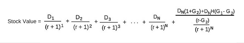
In the above formula, D1 is the value of the next yearly dividend and G2 is the final, stable dividend growth rate. The number of years for which the initial growth rate remains constant is represented by N, while H represents one-half of the duration of the transitionary period. The expected rate of return is represented by r.
Example
To properly illustrate the three-stage dividend discount model, it helps to first work through the formula and then break down the process into the three component phases. This example will expand on the example given in the article on the H-Model using the dividend history of Lockheed Martin (LMT ). In recent years, Lockheed’s dividend growth rates have decreased by about 2.8% per year. Prior to this, however, dividend growth was strong, though erratic. For the four years prior to the current transitionary period, Lockheed’s dividends increased by between 10% and 34%, for an average increase of 19.4% per year.
For the purposes of this example, let’s assume that dividends grew 18.4% each year for four years beginning in 2009, after which the growth rate declined by 2.8% a year for an additional three years before stabilizing at 7.2% in 2017. The result of this calculation will be an estimate of LMT’s value in 2009 based on ‘projected’ dividend activity.
Using the above formula, the dividend information can simply be input where appropriate to yield the value of LMT stock. The initial growth rate covers four years, so N = 4, while the transitionary period is three years, so H = 1.5 The expected rate of return is assumed to 10% and the ‘current’ dividend in 2009 is $2.28. The expected dividends for 2010-2013, therefore, can be calculated as follows:
- D1 = $2.28 * 1.0184 = $2.70
- D2 = $2.70 * 1.0184 = $3.20
- D3 = $3.20 * 1.0184 = $3.79
- D4 = $3.79 * 1.0184 = $4.49
Next, let’s look at the three stages of dividend growth separately. In the first stage, dividends grow by 18.4% per year for four years. The actual dividends for 2010-2013 have already been calculated above:
- D2010 = $2.70
- D2011 = $3.20
- D2012 = $3.79
- D2013 = $4.49
The total value of dividends during the three-year transitional period can be calculated by applying the decreasing growth rates of 15.6%, 12.8%, and 10%:
- D2014 = $4.49 * 1.156 = $5.19
- D2015 = $5.19 * 1.128 = $5.85
- D2016 = $5.85 * 1.100 = $6.44
The value of all future dividends can be calculated using the Gordon Growth Model and the stable growth rate of 7.2%.
- VDFuture = D2016 / (R – G2)
- = $6.44 * 1.072 / (0.10 – 0.072)
- = $246.56
Next, use the 10% expected rate of return to discount each dividend and find its present value.
- PVD2010 = $2.70 / (1 + 0.10)1 = $2.45
- PVD2011 = $3.20 / (1 + 0.10)2 = $2.64
- PVD2012 = $3.79 / (1 + 0.10)3 = $2.85
- PVD2013 = $4.49 / (1 + 0.10)4 = $3.07
- PVD2014 = $5.19 / (1 + 0.10)5 = $3.22
- PVD2015 = $5.85 / (1 + 0.10)6 = $3.30
- PVD2016 = $6.44 / (1 + 0.10)7 = $3.30
- PVDFuture = $246.56 / (1 + 0.10)7 = $126.52
Finally, sum the present values of all future dividends to render the intrinsic value of LMT’s stock in 2009, based on the ‘expected’ dividend performance.
- Stock Value = $2.45 + $2.64 + $2.85 + $3.07 + $3.22 + $3.30 + $3.30 + $126.52
- Stock Value = $147.35
You may note that there is a slight difference between the two calculations due to rounding. For this reason, the use of an online calculator or spreadsheet-based formula is preferable because hand calculations produce greater rounding errors as the number of years of dividend growth increases.
Interpretation
In 2009, LMTs actual market price oscillated between $58 and $85, so this model would have pegged the stock as woefully undersold. An alternative explanation would be that either the expected growth rates were too high or the market actually demanded a rate of return greater than 10%. This example is based on actual dividend data, and the discount rate is considered fairly standard, so in hindsight we know the stock to be undervalued. This holds especially true since it has experienced such healthy growth since 2009, resting comfortably above $200 since July 2015. It is likely that the four years of extremely generous dividend growth – going as high as 33% in 2012 – were unexpected by investors and analysts alike which could have contributed to the stock’s conservative valuation.
Of course, no predictive model is completely accurate and there would have been no way for an investor in 2009 to perfectly predict LMTs dividend activity for the following eight years, especially given its erratic dividend growth in the early 2000s. Nevertheless, had an investor chosen to purchase shares of LMT based on a three-stage calculation like this one, the resulting profits – from both dividends and capital gains – would have been well worth the risk.
Check out the H-Model, the Two-Stage Dividend Model and the Dividend Discount Model.
Image courtesy of adamr at FreeDigitalPhotos.net